What hardware counters can and cannot tell us

First, the short version. Hardware performance counters, the small tallies a processor keeps of what it did while a program ran, are widely proposed as a cheap substitute for actually running an application. I profiled eight applications across 191 configurations on ARCHER2, the UK’s national supercomputer, repeated the campaign on Cirrus, a second machine, and built a tool I called a measurement ladder to work out which part of the measurement was producing the accuracy. Profiling means running a program under a tool that records those tallies. Almost all of it came from one counter (the cycle count), which can only be obtained by running the exact job whose runtime is being predicted, hence the pipeline explains runtime and does not project it. Removing every target-machine measurement multiplies the error by 4.3: with one instrumented run a typical prediction is out by about 13%, and without it by about 56%. Two further results bound the method from above, and both were uncomfortable. Asked to predict an unseen application at an unseen scale, every learned model lost to a two-parameter straight line through the target’s own cheap small-scale runs, and in cross-machine projection, one fitted speedup number per application matched the entire counter apparatus. This was my MSc dissertation at EPCC, supervised by Alexei Borissov.

This is the long version - essentially the dissertation, rewritten for the web. If you want the argument in fifteen minutes rather than an hour, the first four sections and the ladder carry it.

---

Table of contents

Part I. Setting up

1. The question, and why it matters
2. What people already do
3. The four questions I set out to answer
4. The machines
5. The eight applications
6. Five counters at a time
7. The efficiency factor
8. How I decided whether a model was any good
9. The models, and why there are two kinds

Part II. Building it

10. Getting eight codes to run under instrumentation
11. Nine ways the toolchain lied to me
12. What counts as one observation
13. The features, and what they cost
14. A check before any modelling

Part III. Results

15. How to read these numbers
16. Asking a better question
17. The measurement ladder
18. Do the counters earn their keep?
19. The pipeline explains runtime; it does not predict it
20. My p-values are too optimistic
21. Measurement choice dominates model choice
22. Three rounds of neural networks
23. Would more data have helped?
24. The bar is a straight line
25. Transfer between machines
26. Sub-second runs, not Zen 5
27. Pricing the circularity

Part IV. What it means

28. The overfitting warning, revisited
29. Answering the four questions
30. What a practitioner should actually do
31. What I got wrong
32. Limitations
33. What I’d do differently

Appendix

34. Every counter collected
35. The rotation schedule
36. The derived features
37. Source code

---

Part I. Setting up

The question, and why it matters

Two questions come up constantly in high-performance computing, and both need the same impossible thing.

The first comes from a procurement panel choosing between two machines, neither of which is installed. The decision commits several million pounds and shapes what the institution’s researchers can compute for the next five years. Which one runs our codes faster?

The second comes from a user staring at a queue. Their job needs a twelve-hour slot or a twenty-four-hour one, and the two queues have very different waiting times. If they guess low, the job is killed at the wall clock, the time limit the queue gave it, with nothing to show, and if they guess high, it sits behind everything else for a day. How long will it actually take?

Both are asking how an application will perform on hardware before running it there, and the established answers are unsatisfying. Benchmarking directly, which is timing the real code on the real machine, requires the machine to exist and be available, and it burns allocation, the share of machine time a project is granted, on every configuration of interest, a configuration being one application at one problem size on one number of cores. Simulation, which imitates the processor instruction by instruction in software, does not need the machine, but it runs thousands of times slower than it, which confines it to problems far smaller than the ones of interest.

Hardware performance counters suggest a third route. Every modern processor carries a small set of registers, tiny stores of numbers on the chip itself, that count events during normal execution, and they cost essentially nothing to read. The events are things like instructions retired, cache misses at each level, branch mispredictions, and cycles in which the pipeline stalled waiting for memory. In plain words, retired means completed, a cache is one of the small fast memories that sit between a core and the main memory, a branch misprediction is the processor guessing the wrong way at a fork in the code, and a cycle is one tick of the processor’s clock. Critically, they describe how an application uses a machine and not merely how long it took. A code that spends most of its cycles stalled on memory is recognisably different from one keeping its floating-point units, the parts of the core that do arithmetic on real numbers, fully busy, and that difference shows up in the counters.

So it is reasonable to hope the signal transfers. That was the proposal in my feasibility study: profile a suite of benchmarks, relate their counter signatures to runtime, and use the relationship to project performance onto applications and machines outside the training set, the set of examples the relationship was fitted on.

I spent the dissertation testing that proposal. The hypothesis holds, but only in a restricted form, and locating the restriction precisely (quantifying it rather than asserting it) turned out to be the whole contribution.

What people already do

Performance modelling splits into three traditions, namely models derived from a description of the machine, models fitted to measurements, and simulation. It is worth knowing where a counter-based approach sits among them, and in particular how each tradition validates its claims, since the central argument of this project turns on what a validation protocol can honestly support.

Models derived from the machine

The Roofline model (Williams, Waterman & Patterson, 2009) bounds attainable performance by the lesser of peak floating-point throughput and the product of bandwidth and arithmetic intensity, bandwidth being the rate at which memory can supply bytes and arithmetic intensity how many arithmetic operations a code does for each byte it moves. Its cache-aware descendants (Ilić, Pratas & Sousa, 2014; 2017) extend it down the memory hierarchy while splitting the chip into core, uncore and package power domains, and it remains actively applied, including to LULESH, one of the codes profiled here (Afzal, Hager & Wellein, 2025). The uncore is the part of a chip its cores share, such as the memory controller and the last cache before memory.

Roofline predicts a bound rather than a runtime (what a kernel could achieve, not what it will take), which is the essential thing about it.

The Execution-Cache-Memory model (Hager et al., 2013; Stengel et al., 2015) goes further, composing in-core execution time with data-transfer times through each cache level, and Kerncraft (Hammer et al., 2017) automates the analysis. Accuracy is good where these apply. They need a static analysis of the loop nest, meaning the innermost loops where the work happens, read off the code without running it, and a machine model of the target, which restricts them to kernels, single hot loops, rather than whole applications. Later work has had to work hard at abstracting the machine side as processors grew more complicated (Hofmann et al., 2020).

For parallel scaling, the classical bounds (Amdahl, 1967; Gustafson, 1988) and the LogP family (Culler et al., 1993; Alexandrov et al., 1997) are where the standard vocabulary comes from (serial fraction, speedup, and the latency and bandwidth parameters used to describe communication cost). The serial fraction is the share of a program that cannot be split across cores, speedup is how many times faster a run gets when it is given more cores, and latency is the delay before the first byte of a message arrives.

Extra-P (Calotoiu et al., 2013) fits empirical scaling models from a modest number of measurements, and a long line of later work retains most of that accuracy for a fraction of the profiling cost (Ritter et al., 2020; 2026), extends it with neural networks for noise resilience (Ritter et al., 2021), and applies it to distributed deep learning (Ritter & Wolf, 2023).

Extra-P matters more than the others for my purposes. The trend baseline that defeats every learned model I built is a two-parameter version of exactly this idea, and its success here is a small vindication of a well-established line of work rather than a novelty.

Models built from counters

Mechanistic CPI-stack models (Eyerman et al., 2006; 2007; 2011) attack the problem from the measurement side. CPI is cycles per instruction, how many clock ticks an instruction took on average, and a CPI stack decomposes the observed cycles into a base component plus penalties attributable to miss events, with reported errors of 9–13% across three Intel generations. Intel’s top-down method (Yasin, 2014) makes the same idea workable on commodity counters, and it is the approach most likely to be familiar to anyone who has used a modern profiler, the tool that records where a program’s time goes.

The efficiency factor $\eta$ that carries this whole project belongs to that family, and it is much cruder: one scalar, a single number, where a CPI stack itemises. I make no novelty claim for the quantity itself, and what is new here is what I do with it.

All of this rests on being able to read counters portably at all, which is largely down to PAPI, the library that gives every processor’s counters the same names and the same way of reading them (Browne et al., 2000). The reliability of counters has itself been the subject of sustained scrutiny, including a rather bracing survey of the pitfalls in using them for security work (Das et al., 2019). Energy counters have had similar treatment (Hackenberg et al., 2015), and I inherit those limitations wholesale by using RAPL, the processor’s own energy meter.

Models fitted to data

The machine-learning literature replaces the machine model with a fit. Instead of reasoning about caches and bandwidth to derive what performance ought to be, this tradition collects many examples of runs together with their measured runtimes and fits a general-purpose function.

The gain is that no understanding of the hardware is required, and any measurable quantity can be thrown in as an input. The cost is that the fitted function offers no explanation of itself, and no guarantee of behaving sensibly outside the range of the examples it was fitted to.

Reported errors cluster between 10% and 20% (Ding et al., 2020; Sun et al., 2020; Owenson et al., 2019; Malakar et al., 2018), which is a useful yardstick for the ~5% figures I report later, and a reminder that a good-looking number is not automatically a meaningful one.

Regression-based scalability prediction has its own line (Barnes et al., 2008; 2010), as does the configurable-software branch, where deep networks (Ha & Zhang, 2019) and careful sampling strategies (Kaltenecker et al., 2019; 2020) both feature.

Two results deserve particular attention, because they bracket what I attempted.

Marathe and colleagues (2017) used transfer learning (taking a model fitted on plentiful cheap data and adjusting it with a small amount from the setting actually of interest) to identify good configurations from as little as 1% of target-scale observations. That is the cheap-measurement argument in its strongest form, and a related exploratory analysis maps when such transfer works and when it does not (Jamshidi et al., 2017).

Ardalani and colleagues (2015) predicted GPU performance from CPU-only executions, which is genuine prediction of unrun work and precisely the thing this project turns out not to do. Cross-platform prediction has other approaches too, from partial execution (Yang et al., 2005) through representative-region evaluation (Ferrerón et al., 2017) to recent hybrid methods (Mahdavi, 2024), and work predicting new workloads from public datasets (Wang et al., 2018).

On proxy applications

Three of my eight codes are proxies, small programs written to stand in for a large production code by working the hardware the way it does, so the literature on whether proxies represent their parents matters directly to how far my results generalise.

The case for mini-applications was made early (Heroux et al., 2009) and assessed at length since (Barrett et al., 2015). The verdict is broadly encouraging with real caveats: proxies track their parents reasonably well for computation and memory behaviour, less well for communication, and with mismatches that are specific rather than systematic (Aaziz et al., 2018; 2019; Richards et al., 2020). More recent work argues the whole proxy approach needs rethinking for modern workloads (Matsuoka et al., 2022), and kernel-level similarity between proxies and parents remains an active question (McKinsey et al., 2026).

No result here assumes a proxy’s behaviour stands in for its parent’s. The individual proxies I used, LULESH (Karlin et al., 2013) and CoMD (Pearce et al., 2019), have their own characterisation literature, as do the benchmarks STREAM (McCalpin, 1995), HPL (Dongarra et al., 2003) and HPCG (Dongarra et al., 2015).

How this field validates itself

One methodological ancestor shaped this project more than any modelling paper.

Hoefler and Belli (2015) surveyed 120 papers across three major HPC conferences and found it frequently impossible to tell whether a reported improvement was deterministic or a fluctuation. Their recommendations (report distributions rather than point estimates, prefer non-parametric tests, and state the protocol explicitly) shaped the reporting in everything below, where every headline median carries a bootstrap interval and a per-application breakdown. A non-parametric test assumes nothing about the shape of the noise, a median is the middle value of a set of numbers, and a bootstrap interval is a range found by resampling the data many times over to see how far the number can move.

It is also why the superseded results stayed in my working repository rather than being deleted, each with a note explaining what was wrong with it.

Where this work sits

By model class, nothing here is new (standard regressors, the kind of model that fits a number to a set of inputs, on standard counters, and an efficiency factor that is a coarse CPI stack).

The difference is in what the project measures about itself. The studies above report one accuracy figure for a pipeline taken whole, whereas the ladder I describe below attributes that figure between rungs of increasing measurement cost, and here the attribution changes the conclusion.

One recent paper is a close methodological relative. Orteu Aubach and colleagues (2026) merge traces from runs carrying different counter sets, extending coverage past the hardware limit, and report that merged counters retain acceptable accuracy depending on the application. I arrived at the same tactic independently, for the reasons given below, and I also quantify what it costs to merge badly, which turns out to be the story behind this project’s largest retraction.

The four questions I set out to answer

The feasibility study asked a great deal of one fitted relationship: that it hold for applications outside the training set, survive a move to a different machine, and extend to configurations nobody had run. Those are separate demands. A model can meet the first and fail the others, and knowing which it meets is more useful than a single verdict.

• RQ1 - Can application runtime be predicted from hardware counters accurately enough to be useful, when tested on applications absent from the training set?
• RQ2 - How much does each layer of measurement contribute, from free job metadata through a single counter to a full multi-run profiling campaign?
• RQ3 - Does any relationship found transfer to a second machine?
• RQ4 - Can the method predict configurations that have not been run?

RQ2 was not in the proposal. I added it partway through, once it became clear that the accuracy figure I was preparing to report said nothing about which part of the measurement had earned it. That turned out to be the question worth asking, and its answer reframes the other three. An accuracy figure that survives an unseen application counts for little if what produced it was a measurement taken on the very run being predicted.

The machines

Everything was profiled on ARCHER2, the UK national supercomputer, and then again on Cirrus, EPCC’s smaller machine.

Cirrus was replaced during the project by a Turin system, which had two consequences. PAPI works on the new hardware, so the feasibility study’s conclusion that Cirrus counters were unavailable no longer held, and that is the only reason cross-platform work was possible at all. Less helpfully, a 288-core node, a node being one computer in the machine, cannot be matched configuration-for-configuration against a 128-core one, and my first attempt to do so was wrong in a way I’ll come back to.

Everything is single-node by design. The relationship of interest is between microarchitectural behaviour, meaning how a code uses the innards of one processor, and runtime, and multi-node runs would add the effects of the interconnect, the network between nodes, without enriching a counter signature that is collected per rank in any case. A rank is one process of a parallel program, and the processes pass messages to each other through the MPI library.

The eight applications

The suite had to span the space of computational behaviour rather than sample one corner of it, because a model trained on eight codes that all stress memory the same way learns nothing about codes that don’t.

The five primary codes

STREAM is the standard synthetic memory-bandwidth kernel (four vector operations over three arrays, with no meaningful floating-point work and no reuse), and it is the bandwidth-bound corner of the Roofline plane, meaning its speed is set by how fast memory can feed it. I compiled it with three arrays totalling 1.9 GB, comfortably larger than the EPYC 7742’s last-level cache, so the kernel cannot be served from it.

HPL solves a dense linear system, many equations in many unknowns with few zeros among the coefficients, by LU factorisation, the standard way of splitting such a matrix into two triangular ones, and it is the compute-bound opposite corner, its speed set by the arithmetic units rather than by memory. I linked it against Cray LibSci so the inner kernel is a vendor-tuned DGEMM, the dense matrix multiplication routine, rather than the plain reference BLAS, which is what makes it a credible ceiling rather than a badly optimised loop nest. At 128 cores it retires around 4.7 × 10¹¹ floating-point operations while STREAM retires 5.3 × 10⁸, a ratio of nearly 900.

That spread is the point, because leave-one-application-out validation, testing each model on a code it was never fitted on, only means something if a held-out code is genuinely unlike the ones the model trained on.

HPCG is the sparse conjugate-gradient benchmark introduced as a deliberate counterweight to HPL: a multigrid-preconditioned solve dominated by irregular memory access, halo exchange, the swapping of boundary values between neighbouring ranks, and short vector lengths. Sparse means most entries of its matrices are zero, and conjugate gradient is an iterative method that improves a guess step by step. It is the only code in the set that is simultaneously memory-bound and communication-bound, its speed set as much by how fast ranks can talk to each other as by memory, and at 20.8–155.5 s the longest-running. It contributes the most rows of any application, which is why its influence on pooled statistics comes up repeatedly below.

GROMACS is a production molecular-dynamics code, which simulates how atoms move over time, and the only full application here with a genuinely heterogeneous internal structure. It has hand-vectorised short-range kernels that are compute-bound, a long-range part called PME that is bound by Fourier transforms and communication, and the periodic rebuilding of the list of which atoms are near which, which is neither. It is the most expensive code in the campaign at 145–215 s per run, and consequently the most thinly sampled at 26 rows. The benchmark input is a 2,136,412-atom ribosome system.

OpenFOAM is a framework for computational fluid dynamics, which simulates how fluids flow, built on the finite-volume method, and I ran the motorBike tutorial under simpleFoam. Its interest is that it is C++-heavy, indirection-heavy and cache-unfriendly in a way none of the other codes are, indirection meaning that it reaches its data through pointers rather than in straight runs. It is also the one application profiled dynamically rather than statically, at launch rather than by rewriting the binary, because it exists only as a site-installed module, a pre-built copy the centre provides, that cannot be rebuilt. That asymmetry in instrumentation method is a confound, something that changes along with the thing being studied and muddles the reading, and I treat it as one.

The three proxies

I added three Mantevo/ECP proxy applications to cover patterns the original five missed, and to raise the number of distinct applications from five to eight. That matters more than it sounds: the learning curve below shows application count, not configuration count, is the binding constraint.

miniFE is an implicit finite-element mini-application, finite elements being the method that cuts a shape into small pieces and solves on each. It is the cheapest code in the set (0.17–7.0 s) and has by far the lowest floating-point density, making it the clearest case of a code whose runtime is set by data movement and integer address arithmetic rather than arithmetic throughput.

LULESH is a proxy for shock hydrodynamics, the simulation of matter under sudden pressure, of the Lagrangian kind, where the mesh moves with the material, and it is the only code constrained to cubic rank counts. It requires $n^3$ ranks, so it was swept at 1, 8, 27 and 64 cores rather than the powers of two used everywhere else, which is a genuine irregularity in the design.

CoMD is a classical molecular-dynamics proxy standing in for codes like LAMMPS. Its role is to give a second, far cheaper MD signature alongside GROMACS (the same algorithmic family, with two orders of magnitude less work per run), which is precisely the contrast needed to test whether the model has learned molecular dynamics or has learned GROMACS.

The eight codes are not eight independent draws, and I want to state that plainly rather than bury it. miniFE and HPCG are both sparse iterative solvers on regular grids, CoMD and GROMACS are both molecular dynamics, and LULESH and OpenFOAM are both explicit or segregated solvers on unstructured meshes. The effective number of distinct behavioural families is nearer five than eight, and that is the right way to read every leave-one-application-out result below.

The code that got away

CP2K was attempted and dropped. It calls MPI_Init_thread internally in a way that collides with CrayPat’s dynamic instrumentation, and the site-installed module cannot be rebuilt to use static instrumentation instead. I record it because it is a genuine limit on the method rather than a local inconvenience: some applications cannot be profiled this way at all.

BabelStream was considered and skipped for a different reason. It duplicates STREAM’s memory-bandwidth signature, so it would have added rows without adding a kernel. Rows are cheap, and distinct kernels are what the model actually needs.

Five counters at a time

The EPYC 7742 exposes five hardware counters at once, and that constraint shapes everything downstream. A request for more fails at runtime rather than silently multiplexing.

The alternative (multiplexing) was available, and I turned it down. Multiplexing time-slices several counters onto one register and scales up the partial totals, and on a run with phase behaviour those extrapolated counts can be badly wrong. I wanted measurements I could trust, hence each configuration was run five times over with five rotating counter sets:

IPC is instructions per cycle, a FLOP a floating-point operation, prefetching is the core fetching data it expects to need before it is asked, and the TLB is the small table a core uses to translate memory addresses. The sets are not quite disjoint (the cycle count is requested by four of the five, because it is needed to normalise whatever else that run measures). The union covers twenty counters on ARCHER2, of which eleven are also available on Cirrus, and it is that intersection which carries every cross-platform result.

Energy and L3 data come free, because those components have their own registers and are therefore recorded on every one of the five runs rather than one in five. Since the PAPI L3 presets, its ready-made counter definitions, are unavailable on this processor, the Zen uncore component is the only source of L3 information at all, L3 being the last and largest cache before main memory.

Running each configuration five times also yields five wall-clock samples, but they are not replicates, repeated measurements of one thing under the same conditions, and it matters. Each carries different instrumentation and therefore potentially different overhead, so their spread mixes run-to-run variance with instrumentation effects and cannot be read as either alone. An uninstrumented repeat set would have separated the two. I did not collect one, and that is a real gap.

That spread bounds what any result here can resolve. Across the 191 configurations, the ratio of longest to shortest wall time within a configuration has median 1.268 and ninetieth percentile 4.576, the value nine tenths of configurations fall below, with a worst case of 32.9. The large values concentrate in the sub-second runs, where a fixed per-launch overhead of a few hundred milliseconds is a large fraction of the total, and above about ten seconds the ratio is close to 1. Since the effects measured below are of order 0.01 in error factor, this spread (and not the choice of estimator) is the dominant uncertainty in the campaign.

The sweep

The campaign varies three things, namely core count (1, 2, 4, 8, 16, 32, 64 and 128, with Cirrus adding 288), problem size (up to four values per application), and the MPI-to-OpenMP split, which varies at fixed core count for HPCG and miniFE. That split is how the cores are shared between separate ranks and threads inside a rank, OpenMP being the way one program spreads its work across the threads of a node. That gives 191 distinct configurations.

The problem-size axis was a later addition, and adding it fixed a real design flaw. In the first version, each application ran at exactly one size, which perfectly confounded application identity with problem size, hence a model could score well by recognising eight fixed operating points while learning nothing about hardware. GROMACS and OpenFOAM still sit at one size each, and that limitation persists into the results.

The efficiency factor

CrayPat reports counters for rank 0 only, so every counter here describes one MPI rank’s view of the job rather than a sum over ranks.

Rank-0 cycle count is very tightly related to wall time (over the 191 merged configurations the correlation of their logarithms, a number that reaches 1 when two quantities move in lockstep, is $r = 0.993$), but runtime is not simply cycles divided by peak clock. The effective clock implied by $C/t$ ranges from 1.98 GHz for GROMACS, which keeps rank 0 busy, down to well below 1 GHz for STREAM at high core counts, where rank 0 waits on memory.

So I decompose runtime as

$$t = \frac{C}{f\,\eta}, \qquad \eta = \frac{C/f}{t} \in (0,1]$$

with $C$ the rank-0 cycle count, $f$ a fixed nominal reference clock, and $\eta$ a dimensionless efficiency factor absorbing stalls, imbalance and communication. Across ARCHER2, $\eta$ has median 0.807.

Physically, $\eta$ is the fraction of the wall clock during which rank 0 was retiring cycles at the reference rate. The quantity $C/f$ is how long the run would have taken if the processor ticked at exactly $f$ throughout and rank 0 was never held up, whereas $t$ is what actually elapsed. So $\eta = 0.8$ says four fifths of the wall clock was accounted for by cycles at the reference rate, and the remaining fifth went somewhere the cycle count cannot see (rank 0 blocked in an MPI call, the clock running below nominal, or time inside process startup).

Two consequences of writing runtime this way carry the whole project.

The first is that this is an identity, not an approximation. $\eta$ is defined as $(C/f)/t$, so $t = C/(f\eta)$ holds exactly for every configuration by construction, and no modelling assumption is buried in it.

The second is that it splits the problem into a large easy part and a small hard part. The magnitude of the runtime (whether a run takes a tenth of a second or two hundred) is carried entirely by $C$, and $C$ is measured, so nothing has to predict it. Everything left to predict lives in $\eta$, a dimensionless number in a narrow band. That is the whole reason runtime is modelled through $\eta$ rather than directly: it hands the models a bounded, scale-free target instead of one spanning four orders of magnitude.

The convention for $f$ needs stating precisely, because $\eta$ inherits its scale. ARCHER2 runs its EPYC 7742 at a fixed 2.25 GHz. Cirrus’s EPYC 9825 does not run at a fixed clock, and I use its 3.71 GHz maximum boost, the highest speed it reaches when it has the headroom, giving the operative ratio $f_{\text{cir}}/f_{\text{a2}} = 1.649$. So $f$ is a nominal reference rather than an achieved clock, and $\eta$ is a relative efficiency measure whose absolute scale follows that choice (a different Cirrus reference would rescale every Cirrus $\eta$ by a constant). Every comparison below is either within one machine, where the choice cancels, or on the spread of $\log_{10}\eta$, which a constant rescale leaves unchanged.

One more decision was that models predict $\log_{10}\eta$, not $\log_{10} t$. Regressing runtime directly, which means fitting the models to runtime itself, failed badly, doing worse than a constant, and one linear model predicted 6 milliseconds for a run that took 6.1 seconds. Predicting $\eta$ removes the magnitude term, which is trivially available from the cycle count, so whatever skill remains is attributable to the counters.

How I decided whether a model was any good

A fitted model has to be scored on data it was not fitted to, otherwise the score only says how well it memorised. The usual arrangement is to split rows at random. That is exactly the wrong split here, and everything below is conditioned on why.

Models are validated by leave-one-application-out, where I train on seven applications, test on the eighth, and repeat eight times.

A random split would put STREAM at 32 cores in training and STREAM at 64 cores in test, which are near-duplicates on a smooth curve (the same code and the same problem, one step along an axis where behaviour changes slowly and predictably). A model that had seen STREAM at 16, 32 and 128 cores could get STREAM at 64 nearly right by reading off a value in between, without having learned anything about how counters relate to efficiency, and it would be scored as a success.

Holding out a whole application removes that possibility. When STREAM is the test application, no STREAM row of any kind is in training, so there is nothing to interpolate between, and the model must reach the held-out code from seven codes with different algorithms, different bottlenecks and different counter signatures. This is harsher and produces worse numbers, and that is the intended effect.

Error is reported as a symmetric multiplicative factor:

$$\varepsilon = \max\!\left(\frac{\hat t}{t},\, \frac{t}{\hat t}\right) \ge 1$$

Taking the larger of the two ratios means that whichever way the mistake goes, the reported figure is above 1 (predicting 2 seconds for a 1-second run and 1 second for a 2-second run both score 2.00).

Runtimes here span 0.1 to 215 seconds, hence an absolute error would be dominated by the two slowest codes. A tenth of a second missed on a 200-second run is a triumph and on a 0.2-second run is a disaster, yet both are 0.1 seconds. A signed percentage would treat over- and under-prediction asymmetrically, since under-prediction is confined to −100% to 0 while over-prediction is unbounded.

I report both the median and the ninetieth percentile, because they often disagree about which model to prefer: the median describes the typical configuration, p90 the bad ones.

Collapsing the direction does discard information, and it is fair to ask whether a signed variant would change any conclusion. It would not change the comparisons (every model is scored on the same metric), but it would say something these results cannot, namely whether the residuals, the errors left over after the fit, are systematically optimistic or pessimistic. Since $\eta$ is bounded above by 1 in principle, there is a structural reason to expect asymmetry. A signed variant is a cheap addition to any repeat of this work, and it cannot be recovered retrospectively, because the sign is discarded when the error factor is formed.

The statistics

Comparisons below are paired: each configuration is predicted by both methods and the difference is taken per configuration, so the comparison is not disturbed by some configurations being intrinsically harder than others. Three pieces of machinery act on those differences, each chosen to avoid an assumption the data would not support.

The Wilcoxon signed-rank test supplies the $p$-value, the probability of seeing a difference at least this large if there were really none. It ranks the paired differences by magnitude and asks whether positive and negative differences are distributed across those ranks the way they would be if each sign were a coin toss. Because only ordering enters, it needs no assumption that differences follow a bell curve, which matters here, since error factors are bounded below by 1 and unbounded above. It also means a single freak configuration cannot swing the result (it contributes the top rank and no more).

The Holm correction handles multiple comparisons. If twenty independent tests are run at 0.05, the probability of at least one false alarm is about 64%, even if nothing is going on. Bonferroni’s fix is safe but blunt. Holm is a step-down refinement that rejects at least everything Bonferroni would and usually more, and it stays valid when comparisons are dependent, as these are, because they share a baseline.

The Hodges-Lehmann pseudomedian supplies direction and effect size. It takes the paired differences, forms the average of every possible pair of them, and takes the median of those averages. It looks like a strange quantity to compute, but it is precisely the location statistic the signed-rank test is built around, so the reported direction and the reported $p$-value cannot contradict each other.

That last property is not academic. In an earlier version of this analysis I read directions off a difference of two separately computed medians, and seven of twenty-eight came out backwards.

Bracketed intervals are percentile bootstrap 95% confidence intervals. The effect size $r_{rb}$ is the matched-pairs rank-biserial correlation, essentially the win rate rescaled to run from −1 to +1, where negative means the model beats its baseline.

The models, and why there are two kinds

Three estimators appear below: a random forest, a gradient-boosted ensemble, and a multi-layer perceptron. They fall into two families by the only distinction that matters: the shape of function they can represent. The forest and the boosted ensemble are both built from axis-aligned trees and can produce only staircases of flat values. The perceptron produces a smooth curved surface.

Gradient boosting is therefore a second instance of the tree family rather than a third kind of model, and that is exactly why it is useful. When all three land within 0.02 of one another, two of them agreeing is unremarkable and the third agreeing is not.

All three do the same narrow job: take twenty-one numbers describing one configuration, return $\log_{10}\eta$. Runtime is then reconstructed arithmetically as $\hat t = C/(f\hat\eta)$, which involves no model at all.

A decision tree is a flowchart of yes/no questions, each about one feature. At the top sits a single question (is the analytic time below 0.45 seconds?), and a configuration is sent left or right. Each branch leads to another question or to a leaf holding a number: the tree’s prediction for everything arriving there. The questions are not chosen by hand. At each node the fitting procedure tries every feature at every threshold and keeps whichever split leaves the two resulting groups with the least internal spread.

A random forest exists because one tree is unstable. If a handful of training rows move, the question at the top can change, and everything below it changes with it. The remedy is to grow many trees that deliberately disagree, then average them. The disagreement is manufactured by giving each tree its own bootstrap resample (a set of the same size drawn with replacement, so about a third of the training configurations are absent from any given tree), and here 400 trees are averaged.

One property of a forest matters more than any other here, and it is a limitation. Every value a tree can return sits in one of its leaves, and every leaf value is an average of training targets, hence a forest can only return a number inside the range of $\log_{10}\eta$ it was shown. Its prediction surface is a set of flat boxes with jumps between them, and the walls always run at right angles to the feature axes. It cannot extrapolate. Shown a configuration beyond anything it has seen, it hands back the value of the nearest box it already has rather than continuing a trend. That makes it the obvious suspect when I later ask the models to predict at core counts above anything in training.

The random forest. Above: the same feature vector goes to all 400 trees, each grown on its own bootstrap resample so the trees disagree. Their 400 values are averaged, and the resulting η̂ divided into C/f gives the predicted runtime. Below: one tree, where a configuration answers one yes/no question at a time until it reaches a shaded leaf. Thresholds and leaf values are illustrative, though the root feature is the one that does dominate in practice, and the direction is physical: short runs carry a fixed overhead and so a low efficiency factor.

A multi-layer perceptron arrives at its answer completely differently. Rather than asking about features one at a time, it forms weighted sums of all of them at once, passes each sum through a nonlinear activation, a simple bend such as clipping everything below zero to zero, repeats through a second layer, and produces $\log_{10}\eta$. The nonlinearity is not decoration: without it the network collapses algebraically into a single weighted sum and can represent nothing a straight line cannot.

At this size there are over a thousand fitted weights and only 191 training rows, which would let the network reproduce the targets exactly and learn nothing, hence a penalty proportional to the sum of squared weights is added to stop it.

each line carries one fitted weight · information flows left to right

The multi-layer perceptron, end to end. Along the top is the preprocessing shared by every model (median imputation, a signed log compression, then rescaling to mean zero and unit standard deviation). Only a few of the 21, 32 and 16 units are drawn, and cross-platform work narrows the input layer to 14 features and changes nothing else.

Why both are in the project. The forest and the MLP are here as a contrast of functional form rather than as competitors for a prize. If the true relationship between counters and $\eta$ were smooth, and the forest were quietly losing accuracy because it can only build staircases out of it, an MLP would reveal that by pulling clearly ahead.

It does not. All the families land within 0.02 of each other, and that null result is what licenses the claim that measurement choice dominates model choice. Without at least one model from a genuinely different class, the claim would be much weaker: it would establish only that several kinds of tree ensemble agree with one another, which they might well do for reasons of their own.

---

Part II. Building it

Getting eight codes to run under instrumentation

Everything was compiled with the Cray toolchain and instrumented for CrayPat, the profiler that comes with the machine, which means each binary was prepared so that the profiler could count what it did, and the choice of instrumentation method is forced rather than free.

pat_build rewrites the binary statically and gives the richest data, but only if the binary was compiled with the perftools module loaded, which is why GROMACS is built from source here rather than taken from the site module (that module was not built that way). pat_run instruments dynamically at launch and works on unmodified binaries, which is how OpenFOAM is handled, but it is not a universal fallback (CP2K fails under it).

Each job under Slurm, the scheduler that hands out the machine’s nodes, runs one configuration five times, re-exporting the counter selection and a fresh experiment directory between invocations. Two practical constraints shaped this harness. The standard QoS, the queue’s quality-of-service rules, allows only 64 queued and 16 running jobs per user, and bulk submission past that limit fails silently, so a drip-feeder submits from a worklist as slots free and records what it has dispatched, which makes the campaign resumable.

Separately, counter sets must be validated on a compute node rather than the login node, the shared front machine users type at, which does not reproduce the failures. One of my five sets was invalid because a TLB-miss event is a derived event that quietly consumes more than one register, and nothing on the login node revealed it.

Getting eight codes to run under instrumentation across eight core counts was more work than instrumenting them. GROMACS would not configure until three unrelated test targets in CMake, the tool that sets up its build, were disabled. OpenFOAM needed scotch, a library that splits a mesh among ranks, in place of the tutorial’s hierarchical grid (without it the case only runs at the six ranks the tutorial hard-codes), plus two further fixes to its initial conditions. HPL lays its ranks out as a grid of $P$ by $Q$ and needs $P \times Q$ to equal the rank count exactly, which I handled by generating a near-square grid per configuration.

Nine ways the toolchain lied to me

A substantial part of this project was spent on getting the measurement to happen at all rather than on modelling, and I record it for two reasons. The first is that the failures are a property of the method rather than of my particular carelessness, since anyone assembling a counter-based dataset on this toolchain will meet most of them. The second is that they bear on the project’s own argument. I price counter collection in node-hours below, but node-hours are the visible part of the cost. The effort here does not appear in any allocation report, and it is not small.

The column that matters is the middle one. In six of these nine cases the message does not point at the fault, and in three there is no message at all.

The pattern here is that silent and misdirected failures are the expensive ones. Three of the nine failures are silent, and a fourth (a stray /tmp/inspect.py left over from earlier testing, shadowing the standard library module of that name) produced the same misleading error as an unrelated NumPy problem it outlived, so that fixing the real cause appeared not to work.

They are expensive because the loop is not edit–error–fix but edit–plausible-looking-output–discover-much-later. That is also the mechanism behind the analysis defects I found and corrected during the project: a rigged baseline and a pseudo-replicated feature matrix both produced entirely reasonable-looking numbers.

The lesson I would carry forward is that on this toolchain, an absent error message is not evidence of success, and the check that catches these is an assertion on the shape of the output rather than on the return code.

Some things were never available. The set of PAPI presets that exist on Rome is narrower than the documentation suggests (several cache-miss presets are simply absent), which is why L3 information comes from the Zen uncore component. Network and node-power counters are disabled on ARCHER2, so communication cost is inferred from per-function MPI timings instead.

What counts as one observation

pat_report emits counter values as formatted text, and parsing it is fussier than expected: a regular expression, a pattern for matching text, that matches the value lines also matches the legend at the foot of the report, which is how I briefly had an L3 miss count of three.

The consequential decision was what counts as one observation (one row of the table the models are fitted to).

I first treated each of the five counter-set runs as an independent row, giving 815 samples. That is wrong twice over.

First, it is pseudo-replication. The five runs are the same configuration executed five times, differing only by run-to-run noise and by which counters were requested, hence counting them as five separate observations claims five times the evidence the experiment actually gathered.

Second, because each run measures only its own five counters, most of each row is empty (0% availability for three features, 50% for IPC, and 44.1% overall). The gaps have to be filled before a model can be fitted, and they were filled by median imputation, which writes the column’s middle value into every gap. That is the least harmful simple choice, but on a column that is mostly missing it produces a column that is mostly one repeated number, with consequences for how the forest distributes feature importance, its own score of how much each input mattered, that I will come back to in a big way.

Merging to one row per configuration (taking the union of counters across the five sets and the median runtime) gives 191 configurations at 97.4% populated. The merge added coverage without any new measurements, and three features observed on no unmerged row carry 0.078 of the importance mass once merged.

One consequence of merging column by column should be stated, because it affects $\eta$ directly. Counter set C requests no cycle count, so the median cycle count is taken over the four runs that measured it while the median runtime is taken over all five. The two medians can therefore come from different runs, and $\eta$ becomes a ratio of medians over different samples rather than the median of a ratio. On 20 of the 191 configurations this displaces $\eta$ by more than 5%, and on one (HPL at size 2000 on 32 cores) it produces $\eta = 1.040$ where the paired computation gives 0.466.

Recomputing $\eta$ per run before merging would remove the artefact and is the correct construction. I did not do it, and the affected configurations are a tenth of the dataset.

The features, and what they cost

A feature is one of the numbers a model is given about a configuration. Twenty-one are derived here, and the raw counters are never used directly: what enters is always a ratio of two of them (instructions per cycle rather than instructions, and L2 misses per instruction rather than L2 misses).

The reason is that a raw count grows with how much work the run did, so a model given raw counts could score well by recognising that a run with many instructions is a long run. That is true and useless, and it is already carried by the cycle count. Ratios divide that magnitude out and leave only the character of the execution, which is the transferable part.

Core, rank and thread counts enter as base-two logarithms, since they double rather than increase in steps.

One magnitude term is retained deliberately: the logarithm of the analytic time $C/f$. Other raw magnitudes are excluded, since several let a model fasten onto problem scale instead of behaviour. One explicit scale covariate, an input that stands for the size of the run, is still necessary, because $\eta$ is strongly run-length dependent (a short run carries the same fixed startup cost as a long one and so looks less efficient), and when the forest is denied it, it splits on a correlate instead.

Retaining it agrees with the ladder rather than contradicting it. That feature is the top of the twenty-one on both measures of importance (impurity importance, which scores how much a feature’s splits tidy the training data, at 0.375, and held-out permutation importance, which scores how much accuracy on unseen data drops when that feature is scrambled, at 0.0150 against 0.0059 for the next feature). The second is the harder test, because it is measured out of fold, on data the fit never saw, and so cannot reward a feature for memorising the training set.

The twenty features beyond it are therefore measured against a model that already holds the cycle count, inside the fit as well as outside it. The question they face is whether they add anything to a model that already knows the analytic time, rather than whether they predict $\eta$.

What the campaign cost

The ARCHER2 sweep comprised 191 configurations, each run five times, plus validation and failed attempts, which came to roughly 1000 profiled executions and approximately 210 node-hours, a node-hour being one node for one hour. The Cirrus campaigns add about 90 more.

The applications themselves account for only about six of those hours. The rest is job startup, queue-slot granularity, post-processing, and the failed and repeated attempts, which is the real shape of a profiling campaign, and part of why the cost argument here is about wall-clock commitment rather than compute.

The twenty features beyond the cycle count cost four fifths of that budget, which is worth stating plainly for a project whose argument is about measurement cost.

Three hundred node-hours is not, in isolation, a large number, and the cost argument rests on how the total scales rather than on the total itself. The figure buys eight applications on two machines, which makes it a cost per application-machine pair that grows multiplicatively with every axis added. Covering the thirty or so codes a mid-sized centre actually runs, across three machines, at the same density, would be an order of magnitude more. The learning curve below says the application axis is the one still paying, so that is the axis a serious campaign would have to extend.

The relevant comparison is also against the alternative rather than a compute budget: the trend fit below needs only a handful of short runs of the one code in question, and it beats every model here.

Model configuration

Random forests use 400 trees with a minimum of two samples per leaf. Gradient boosting uses 300 estimators at depth 3 (shallow enough that each tree is weak on its own), with learning rate 0.05 and a quantile objective matched to the error metric, so the model is fitted to the same statistic the results report. The learning rate is the size of each correction step, and the quantile objective means the fit aims at the median rather than the mean. The MLP searched hidden layers in {(16), (32,16), (64,32)} against an L2 penalty, the weight on the sum of squared weights mentioned above, in {0.1, 1, 3, 10}, giving twelve candidate settings.

These are hyperparameters, which are settings fixed before the fitting procedure starts rather than learned from the data by it. They are chosen by nested selection, a fold being one round of the leave-one-application-out with one application held out. Inside each outer fold, an inner leave-one-application-out loop runs over the seven training applications alone, each candidate is scored on applications the inner loop holds out, and the winner is refitted on all seven and applied to the eighth.

The held-out application plays no part in choosing them. That is the point, and choosing them by looking at how they score on the held-out application is a way of letting the test set into the fit. I measure what that did below.

A check before any modelling

Before trusting anything, I checked the campaign had measured what it was supposed to.

Each application’s median runtime plotted against core count shows three things. First, each code scales the way its algorithm predicts. HPCG is sized per rank, so adding cores adds work, and its ARCHER2 median actually rises from 31.6 s at one core to 46.8 at 128 (the weak-scaling cost of a growing halo exchange), while OpenFOAM scales cleanly from 132.7 s down to 5.0. Weak scaling is the case where the problem grows with the core count.

Second, and this became important later, a shaded sub-second band shows what running Cirrus at ARCHER2’s problem sizes did to the experiment: a quarter to two thirds of Cirrus runs fall into it for CoMD, HPL, LULESH and miniFE (reaching 65% for miniFE). HPCG, alone in being sized per rank, never enters it.

Third, package energy per rank falls monotonically in core count for every application.

One panel does not carry a scaling signal, and it is a defect rather than a finding. STREAM’s expanded-campaign runs sit at 3.3 seconds at every core count because they were launched single-threaded, which I return to in the limitations.

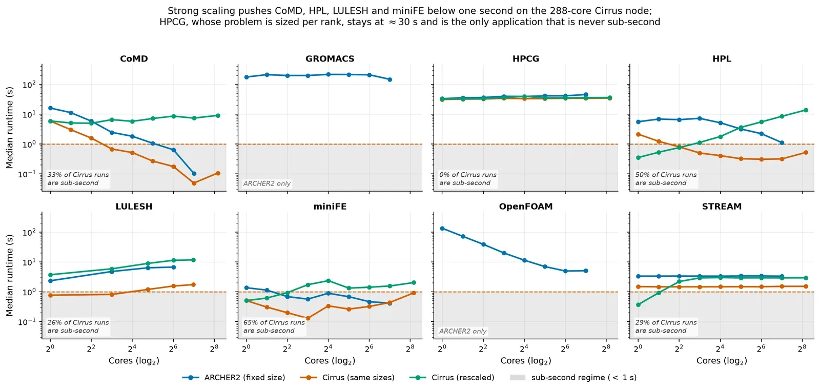
Every code scales the way its algorithm predicts. The shaded band is the sub-second regime, and the orange line diving into it is what copying ARCHER2’s problem sizes onto a 288-core node did to the experiment (65% of miniFE’s Cirrus configurations end up there). HPCG, alone in being sized per rank, never enters it, which is the clue that eventually explained the whole problem.

This is a check on instrumentation and parsing rather than a result, and it passed.

---

Part III. Results

How to read these numbers

Every result below is an error factor: 1.00 is exact, 1.10 is out by ten per cent either way, 2.00 is wrong by a factor of two, and 1.00 is the floor. Alongside the median I report p90, the ninetieth percentile, which describes the bad cases rather than the typical one.

Results are quoted two ways and they can disagree.

A pooled median throws all 191 configurations into one pile, so every configuration counts once, which means an application contributing many configurations counts many times over (HPCG alone supplies 45 of them).

A macro-average takes each application’s own median first, giving eight numbers, then averages those eight, so every application counts once regardless of how many configurations it brought.

The two answer different questions: how does the method do on a typical configuration? against how does it do on a typical application? Because the applications are unequally represented, the answers can differ in size and occasionally in direction. Where they disagree I give both, because the disagreement is usually the interesting part.

Comparisons are paired: the difference is taken per configuration, so what is examined is 191 differences rather than two piles of 191 errors. One consequence matters below. A paired comparison can point the opposite way to a comparison of two separately computed medians, because the median of a set of differences is not the difference of two medians. A method can improve most configurations by a little while a handful of large errors hold its own median up.

Several baselines appear, and it matters which is in play:

• the constant - a single fitted efficiency factor for all applications, 1.065 on ARCHER2, which is the answer obtained by ignoring all twenty-one features. I call it the zero-parameter bar because it fits no coefficients to anything. It reads nothing off the run being predicted, so it is what every model must clear before any profiling can be said to have paid for itself.
• the same-fold constant - the constant computed on exactly the configurations a transferred model is tested on, which is the fair reference for cross-machine work and not the same number.
• the trend fit - a two-parameter straight line through the target application’s own cheap small-scale runs.
• the clock-ratio rescale - predicting one machine’s runtime from the other’s by the ratio of clock speeds alone.
• the circular ceiling - what is achievable when a counter measured on the target run is allowed, which is unachievable in practice and bounds the rest.

The resolution of these numbers

Two sources of variation bound how finely any of this can be read, and I want them stated before the numbers start rather than buried in a footnote.

Across three independently written evaluation scripts, the 21-feature random forest on these 191 rows scores 1.0496, 1.054 and 1.0554: an implementation spread of 0.0030. Refitting one implementation under ten random seeds, the starting points of the randomness inside the fit, spans 1.0497 to 1.0655, a spread of 0.0158, five times larger and the binding one.

Differences below about 0.016 should be treated as noise.

That threshold is larger than two differences I report below: the 0.011 separating the top two rungs of the ladder, and the 0.011 separating the random forest from the constant. Neither survives as a point estimate. Both remain informative as paired comparisons, because those hold the seed fixed and compare per-configuration errors rather than two independently fitted medians, and the conclusions rest on the paired tests and the macro-average rather than on the pooled point estimates.

Asking a better question

For a while I had a pipeline that produced a number, a median error factor around 1.05 (a typical prediction landing within about 5% of measured runtime, for an application the model had never seen). That is a respectable-sounding result and I was preparing to report it.

Then I got uneasy about what it meant, and the unease is the most productive thing that happened in the project.

The issue is that a single accuracy figure for a pipeline says what the pipeline achieves without saying which part achieved it. My pipeline consumed a lot of different measurement (free job metadata, one counter, and five counter sets over five separate runs). If most of the accuracy came from the cheapest part, the expensive campaign was pointless, and if it came from the expensive part, the campaign was justified. The 1.05 figure is silent on that, and it is the question a person deciding whether to do this profiling actually needs answered.

So I stopped asking “how accurate is the pipeline?” and started asking “which part of the measurement is the accuracy coming from?”

The instrument I built to answer it is what I called a measurement ladder: a series of predictors, or rungs, each using strictly more measurement than the one below, all evaluated under one identical protocol. The discipline is entirely in the word identical, meaning the same 191 configurations, the same folds and the same metric. The only thing differing between two neighbouring rungs is the extra measurement the upper one consumes, so any improvement between them is attributable to that measurement and nothing else.

The measurement ladder

The rungs, in order of how much measurement each demands:

• Rung 0 - the training median. It predicts the same runtime for every configuration of the held-out application (the median of the seven training applications’ runtimes), and it measures nothing whatsoever about the target. It exists to establish what knowing nothing scores, so everything above can be quoted as an improvement on something.
• Rung 1 - free job metadata. A random forest given three numbers known before submission (core count, rank count and thread count), with no profiling, no counters and no execution. Along with rung 0, this is the only rung that is a genuine prediction in the sense the feasibility study meant, because it could be evaluated for a job nobody has run.
• Rung 2 - the cycle count alone. It takes $C/f$ and stops there, assuming $\eta = 1$. That is one counter, but that counter comes from an instrumented run of the exact configuration being predicted.
• Rung 3 - cycle count plus one fitted scalar. Rung 2 divided by the median $\eta$ of the training applications, which is one number, fitted once and applied to everything.
• Rung 4 - the full campaign. Rung 2 divided by an $\eta$ predicted by a random forest over all twenty-one counter-derived features, which costs five instrumented runs of the target configuration.

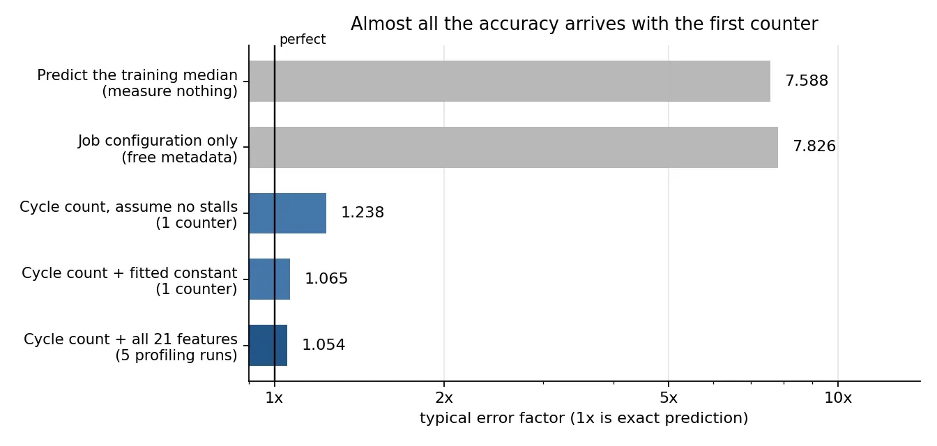
The same table as a picture. Note the log scale: the step from free metadata to a single cycle count is a factor of six, and everything after it is a factor of 1.17.

The total improvement from rung 0 to rung 4 is 6.533 in error factor, and of that, the cycle count alone accounts for 6.588, slightly over 100%. Fitting a constant $\eta$ adds 2.6%, and the twenty remaining counter-derived features add 0.2%.

The share exceeds 100% because rung 1 contributes a negative amount. Free job metadata is worse than useless: under leave-one-application-out, “128 cores, 128 ranks, 1 thread” is all the model has, and nothing in that distinguishes STREAM from GROMACS. A model asked to place an unseen code on a scaling curve from that alone does worse than declining to try, which is the correct answer rather than a modelling failure, because the honest response to being told nothing is to say nothing.

Where the definitional part ends

I want to mark the boundary between the definitional and the empirical part of that result, because a reader could take the 100.8% as the discovery of the project when it is closer to an accounting identity.

Rung 2 is not really a model. The equation $t = C/(f\eta)$ defines $\eta$, so setting $\eta = 1$ restates the definition, and predicting $C/f$ rearranges a measurement rather than inferring from one. Cycle count and runtime are nearly the same quantity (their logarithms correlate at $r = 0.993$), so the cycle count accounts for 98.6% of the variation in log runtime before any modelling happens at all. Rung 3 is definitional in the same sense.

What the ladder does measure, and this part is not definitional, is how small the quantity left to predict actually is. The constant baseline’s 1.065 means a typical configuration’s $\eta$ sits about 6.5% from the median, and that band is all the room any model has. No amount of modelling skill can win more than the gap between predicting one efficiency for everything and predicting it perfectly.

Against a 6.5% band, the twenty features recover a detectable slice. My claim is that the quantity left to predict is small and this experiment says how small, rather than that one counter does everything.

Macro-averaging sharpens the counters’ case

Pooling 191 rows lets HPCG, at 45 of them, speak for a quarter of the result. Weighting applications equally, rung 4 reaches 1.058 against rung 3’s 1.111, five times the pooled gap.

The counters help most where the constant does worst (miniFE and LULESH), and hurt on HPCG, STREAM and OpenFOAM.

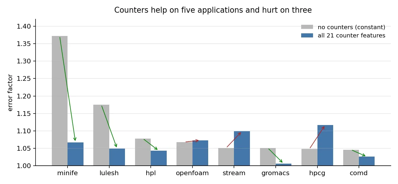
Green arrows mark applications the counters improve and red arrows those they make worse, and the gain is concentrated in the two hardest cases.

Rung 4 is a large gain on five applications against a real regression on three, and that is what bounds any practical claim.

And here is the part that reframed the project

Everything above rung 1 depends on the cycle count, and the cycle count can only be obtained by running the job whose runtime is being predicted.

Do the counters earn their keep?

If the twenty extra features add 0.2% on typical accuracy, was the five-set profiling campaign worth doing at all?

The table below cuts the same experiment by feature group rather than by measurement cost, and adds the significance tests the ladder omits.

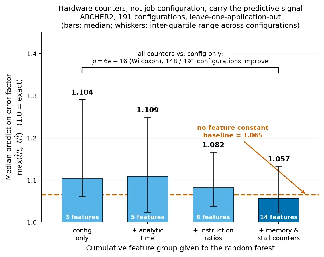
Only the last bar clears the dashed baseline, and the second bar goes the wrong way (adding the analytic cycle term to job configuration makes the model marginally worse, not better).

Read plainly, the full five-set rotation is the only feature configuration that beats a zero-parameter constant. Free metadata is significantly worse than guessing the training median, one counter does not rescue it, and one counter set is still indistinguishable from guessing. Everything cheaper than the full campaign fails.

A second reading is more generous to the counters, and both belong in the record. Relative to free metadata rather than to the constant, every counter rung adds genuine signal. The full set wins 152 of 191 comparisons with a large effect size ($r_{rb} = -0.69$, $p = 6.3 \times 10^{-16}$), and even the single analytic cycle counter is a significant improvement.

So the campaign does earn its keep, but the thing it buys is modest and it only arrives at the end. There is no partial credit here, and no cheap 80% of the benefit for 20% of the cost. You either run the whole rotation or you may as well predict a constant.

The gain also shows up mostly in the tail rather than the middle. Median error moves from 1.065 to 1.050, about one percentage point, but p90 (the error you should plan around) falls from 1.532 to 1.390. The defensible claim is that models cut worst-case error by roughly 17% while a constant suffices for typical cases. For queue-slot sizing, where the whole point is not being caught out by the bad case, that is arguably the number that matters.

The pipeline explains runtime; it does not predict it

The ladder settles what the pipeline is, and tracing exactly which quantities a runtime prediction consumes is what exposes the problem.

Every rung from 2 upwards, including the headline pipeline at rung 4, reconstructs runtime as $\hat t = C/(f\hat\eta)$, where the models supply $\hat\eta$. Nothing supplies $C$. It is read off a measurement, and it is not predicted, estimated or approximated.

Nor is it a measurement of something similar. The analytic term requires the cycle count for the configuration whose runtime is being reported, which means that application at that problem size at that core count on that machine, and not a similar configuration or the same code at a different core count. A hardware counter can only be obtained by running the program and counting events as they happen, hence the cycle count is the product of a completed instrumented run of exactly the configuration whose runtime is being “predicted.”

The circularity follows immediately. Evaluating $C/(f\hat\eta)$ requires having run the job, and once the job has run it has already been timed, because the wall time and the cycle count are printed in the same report, from the same execution. There is no situation in which a practitioner possesses $C$ and lacks $t$.

The 1.054 figure is therefore conditional on having already run the thing being predicted, and cannot be read as a prediction of an unrun execution. This is a statement about the structure of the method rather than its accuracy, hence no amount of extra data or better modelling would change it, and only a different predictor would (one whose inputs do not require the target run).

How much must the profiled run resemble the run of interest?

The circularity is at its most severe when the profiled run is the run being predicted, but that is not the only way to use the method, and the weaker forms are worth separating.

Predicting a different configuration of the same code is genuinely possible. The models are never shown the held-out application, and restricting training to small core counts costs essentially nothing, so a profile at one scale does carry information about another, and only the cheap trend fit beats the models at doing so.

Predicting a different application from a profile of some other code on the same machine is a stronger claim, and it is the one leave-one-application-out tests directly. The counters beat a zero-parameter constant on five of eight applications, so there is cross-application signal, but it is small and it regresses on the other three.

What is not possible in any form is obtaining $C$ for a configuration nobody has run, and $C$ is where essentially all of the accuracy lives.

This does not make the result empty

It makes it a different result. What the pipeline delivers is a decomposition of a measurement: a validated explanation of the gap between the ideal cycles-at-reference-clock time and the observed wall time, expressed through microarchitectural quantities and tested on applications it has never seen.

Explaining and predicting are genuinely different jobs, easily confused because both are reported as the same kind of number. A prediction tells you something you did not have, whereas an explanation accounts for something you did. Knowing that a run took 40% longer than its cycle count implies, and which microarchitectural quantities that shortfall tracks, is useful: it bounds worst-case behaviour, it is validated on unseen codes, and it is honest. But it is not the thing the feasibility study promised.

I established this by building the ladder, not before. Had I only reported the headline 1.054, the circularity would have been invisible in the write-up. The figure looks exactly like a prediction accuracy, is computed exactly as one would compute a prediction accuracy, and is validated on genuinely unseen applications, so nothing about its presentation would give the game away. What exposes it is putting rungs 1 and 2 side by side under one protocol and noticing that the entire improvement arrives at the step where target-run measurement enters.

I suspect the same thing is invisible in some published work for the same reason.

My p-values are too optimistic

Every $p$-value in this article is too small, and I would rather say so than let them stand unqualified.

A significance test assumes its observations are independent, and a test handed 191 rows that really carry the information of far fewer returns a $p$-value more decisive than the data deserve. That is the situation here. The configurations are eight applications × eight core counts × up to four sizes, sitting on smooth scaling curves. Knowing how the forest does on miniFE at 32 cores says most of what it will do on miniFE at 64.

That is the same non-independence I invoked to reject a random train/test split, and I cannot have it both ways. If neighbouring configurations are too alike to be split across training and test, they are too alike to be counted as independent evidence either, hence the effective sample size is nearer eight than 191.

The remedy is to repeat the comparison at the unit that genuinely is independent (the application), and accept the much weaker evidence eight observations can supply.

At application level the random forest beats the constant five times out of eight. A sign test is the appropriate instrument and the crudest available, discarding the sizes of the wins and keeping only their direction. Five or more wins in eight comes up about 36 times in 100 by chance, so $p \approx 0.36$.

Five wins in eight is not a surprising outcome for a method with no advantage at all.

The bootstrap intervals agree. The forest’s [1.037, 1.074] overlaps the constant’s [1.052, 1.081] across most of its range, which means resampling the data moves the two numbers around by more than the distance between them.

So the improvement is consistent in direction, large where it appears, and not established at the unit the validation protocol itself treats as independent. Both units are reported throughout, and the application-level reading is the one that bounds the claim.

The effect is real and small, and it is priced. The practical implication is clean: there is no cheap version of this method. The five-run campaign is the threshold at which the pipeline starts working at all, and not an incremental refinement of a working cheap pipeline.

Measurement choice dominates model choice

Before comparing estimators, there is a result about what a fitted model can and cannot be asked.

The obvious use of a forest is to read off which counters matter most, and hence which hardware characteristics drive runtime. That reading is invalid on an unmerged matrix of the kind counter rotation produces, because impurity importance then tracks how often a counter was observed rather than how much it explains. Under a control that re-imposes the old observation pattern on corrected data, importance and observation frequency correlate at $\rho = +0.798$, a rank correlation, which runs from −1 to +1. Merging to one row per configuration removes the artefact ($\rho = +0.080$).

The diagnosis and the fix are the same operation, and the practical warning is general: any rotated-counter campaign that reports feature importances without merging first is reporting its own sampling schedule. I return to this below, because it is also the story of the project’s largest retraction.

Now the estimators:

The models sit within 0.02 of each other, which is the finding. At this resolution the accuracy does not depend on the choice of estimator. The ranking even depends on which statistic is chosen (the two tree models share the best median, and the ensemble takes the tail), and all the intervals overlap. Against the constant, the random forest wins 125 of 191 at $p = 2.2 \times 10^{-4}$, while the nested-selection MLP is indistinguishable from it. Every one of these gaps is smaller than the 0.016 noise floor, so no ordering among the learned models is claimed.

The MLP is the key line of that table, and it is included to be structurally different rather than to win. If the relationship between counters and $\eta$ were smooth, and the tree ensembles were paying an accuracy penalty for approximating it in steps, the MLP is the model that would show it by pulling ahead. It does not. Two model classes with nothing in common structurally arrive within 0.02 of the same answer, and within 0.02 of a constant. That is a much stronger basis for saying accuracy does not depend on the estimator than agreement among tree ensembles would be, since those might agree simply by sharing the same blind spots.

That table also holds a nice methodological aside. One MLP row was tuned by inspecting the evaluation folds (exactly the contamination you are told to avoid), and it scored 1.076, worse than the 1.063 from doing it properly. The reason is that the contaminated version fixes one architecture across all eight folds, while nested selection chooses per fold, and that flexibility is worth more than the leaked information.

The defect is the invalid protocol, whichever direction it moved the number. An improper protocol that happens to flatter the model less than a proper one is still improper, and the number it produces still cannot be reported as an honest estimate. It is a useful reminder that contamination does not always inflate results, so “the number looks plausible” is not evidence the protocol was sound.

Three rounds of neural networks

Neural networks were pursued through three rounds and were never competitive.

Round one was plain multi-layer perceptrons, and round two was corrected tuning after the first round’s protocol turned out to be contaminated. Round three brought in published state of the art for tabular data (PLR numerical embeddings, robust scaling with smooth clipping, RealMLP and deep ensembling, which are recent recipes for getting neural networks to work on tables of numbers).

Every neural approach lost to the zero-parameter constant, and PLR embeddings (the most-recommended technique in the recent tabular literature) were the worst of the lot, at $p = 3 \times 10^{-6}$.

The mechanism is not mysterious, and identifying it is what makes this a result rather than a failure. There are 191 rows. Modern tabular deep learning methods are developed and benchmarked on datasets two or three orders of magnitude larger, and their advantages appear at that scale. Below it, the extra capacity has nothing to feed on, and worse, 62% of the target lies in a narrow band, so there is very little signal for extra capacity to capture even in principle.

I report it as a negative result with a mechanism attached, because “we tried neural networks and they didn’t work” is only useful if you can say why, and therefore when they might.

Would more data have helped?

A learning curve answers that question without collecting any. The trick is to deliberately throw data away, fitting on a quarter of the training set, then a half, then three quarters, then all of it, and plotting how the error falls. If the curve is still dropping at the right-hand edge, more data would have helped, and if it has flattened, it would not.

Throughout, the test fold is left untouched, so all four points are scored on exactly the same configurations and are directly comparable.

Here “more data” can mean two different things, and the two ways of subsampling give opposite answers. The contrast between them is the result.

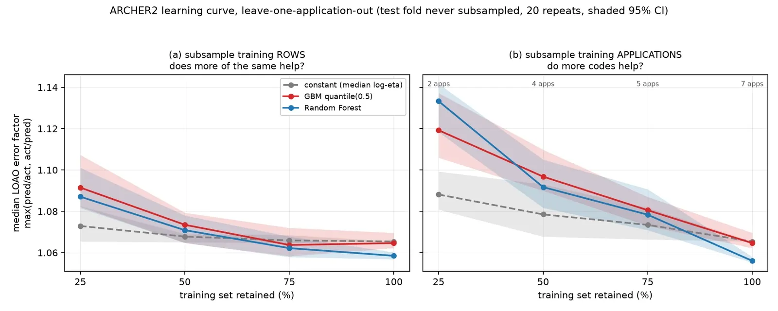
Left: more runs of the same eight codes - the curve flattens, and the data is saturated on this axis. Right: more codes - still descending at the right-hand edge with no sign of levelling off.

Removing training rows at random, the forest improves from 1.0871 to 1.0585, but the last quarter buys nothing resolvable, hence on that axis the dataset is saturated.

Removing whole training applications, the curve is still descending at seven codes, from 1.1333 at two to 1.0560 at seven, with the 75% and 100% intervals disjoint.

This axis also fixes the method’s floor. The constant improves with coverage more slowly, so at two training applications the forest is worse than the scalar, and below roughly four training codes the counters are a liability rather than a weak help.

The binding constraint is therefore the number of applications, and I had the budget allocated the wrong way round. Profiling each code at eight core counts and four sizes bought density the model had stopped using, while the axis still paying got eight. It also means the headline itself is measured on the steep part of that curve, so its stability is limited by coverage rather than by anything about the estimator.

The bar is a straight line

Every result so far holds one axis fixed: leave-one-application-out varies the application while all core counts remain visible. The test matching the feasibility study’s promise crosses both - train on other applications at small core counts, then predict the held-out application at large ones.

The right competitor here is not a constant. It is what a practitioner would actually do with an unfamiliar code: run it cheaply at small scale and extrapolate its own trend. That means plotting log runtime against log core count for a few cheap runs, fitting a straight line (two parameters), and reading it off at the core count of interest, with no counters, no training set, no model and no other applications.

That is a low bar in cost and, as it turns out, a high one in accuracy.

The learned models are behind the trend fit at all three thresholds tested, a threshold being the largest core count the models were allowed to train on.

The evidential strength needs care, because the three thresholds share configurations and cannot be pooled as independent observations. Taken separately, at $T = 8$ the forest is worse by +0.023, not significantly ($p = 0.094$), at $T = 16$ it is significantly worse (+0.032, $p = 0.047$), and at $T = 32$ it is worse by +0.052, not significant ($p = 0.212$). The direction is consistent across all three thresholds and every learned arm, while the significance holds at one of three.

A naive reading would say the forest at 1.113 is worse than the constant at 1.102, but the paired test says the opposite (the forest wins 140 of 240 individual comparisons, $p = 1.5 \times 10^{-5}$). The models do beat a constant. They lose to the cheaper trend fit, which is the comparison that matters.

The reason they lose is not an inability to extrapolate in scale, which was my first suspicion. A forest is confined to the range of its training data, so asking one to predict at 128 cores having seen only 8 is where that limitation should bite. Lifting the restriction tests it. Training on all scales rather than only small ones changes the forest’s error by a factor of 0.993 at $T = 8$, 1.003 at $T = 16$ and 1.034 at $T = 32$, which is under 1% in two cases and in the wrong direction in the third.

So the scale restriction costs essentially nothing. The models were never better than a per-application straight line at any scale. That is a cleaner result than a failure to extrapolate, and it is the most useful negative in the project, precisely because the competitor is so cheap.

Transfer between machines

The cross-platform comparison needed fixing before it could be made at all.

An earlier version of this work claimed 191 matched configurations on each machine (paired row for row, the same application at the same size on the same core count, so the only thing differing between the two numbers is the machine). That was false. GROMACS and OpenFOAM were not tested on Cirrus, and its 288-core node reaches core counts ARCHER2 cannot. Joining properly leaves 166 genuinely matched configurations. The two totals of 191 were a coincidence of how far each sweep happened to run.

Comparing the unmatched sets would have been comparing two differently composed workloads and attributing the difference to the hardware.

The bias had a direction. The 25 unmatched Cirrus rows are its widest and shortest runs (a median runtime of 1.04 s against 1.20 for the matched ones) - exactly the configurations where fixed overhead dominates and $\eta$ collapses. Including them made Cirrus look harder to predict for reasons unrelated to its microarchitecture.

On the paired set, staying on one machine gives 1.071 on ARCHER2 and 1.125 on Cirrus, whereas transferring gives 1.203 going to Cirrus and 1.157 coming back. Transfer costs accuracy in absolute terms, and that is the headline for RQ3.

Against the right baseline, though, the transferred model earns its place. The reference for an ARCHER2 → Cirrus prediction is the constant on the same folds, 1.2203, and not Cirrus’s own within-platform constant of 1.129, which is fitted on Cirrus data the transferred model never sees. Against that the random forest at 1.2025 is significantly better (Holm $p = 0.006$), while coming back the other way, no model beats its same-fold constant of 1.1511.

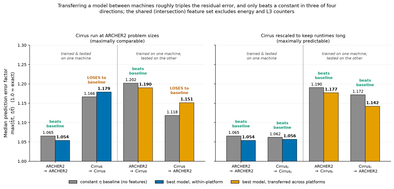
Within a machine, error sits near 1.05, and every crossing lands between 1.14 and 1.19, which is roughly three times the residual error over perfect prediction.

Transfer degrades the models without destroying their advantage over doing nothing, and the asymmetry is real, in that the model trained on the machine with the wider $\eta$ spread transfers worse.

It is worth seeing what a working transfer actually looks like, rather than only its summary statistic:

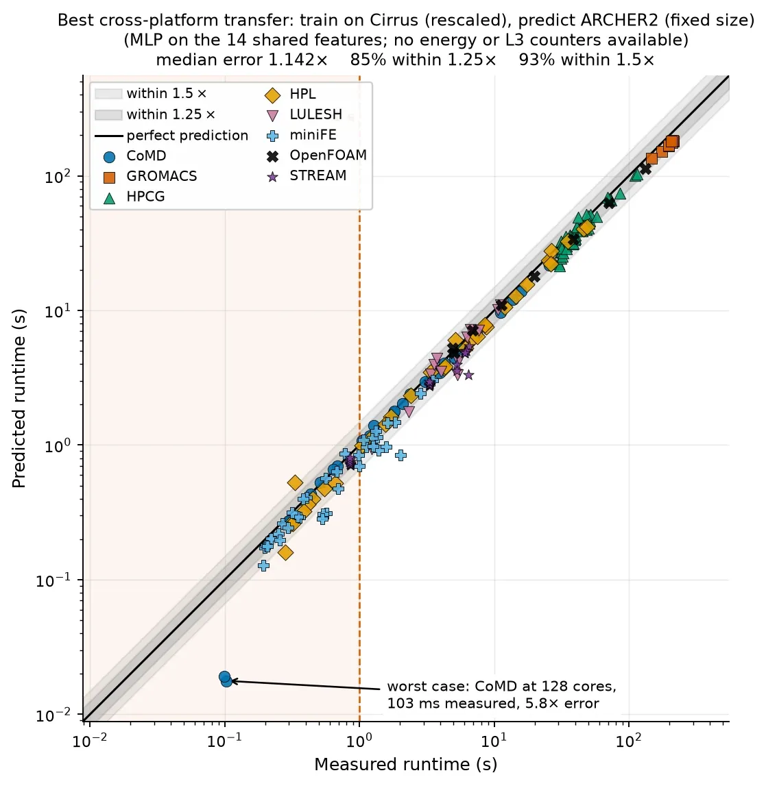
An MLP trained entirely on rescaled Cirrus data, applied without retuning to ARCHER2, using only the fourteen shared features. The median error is 1.142, and 85% of configurations fall within 1.25× and 93% within 1.5×, across four orders of magnitude and eight applications never seen at these problem sizes. Accuracy is uniform across applications (the per-application medians run 1.09 to 1.19).

The single serious failure is the one annotated point, CoMD at 128 cores (a 103 ms run), under-predicted by 5.8×. It sits squarely in the fixed-overhead regime, which is the same mechanism as the sub-second problem below appearing here as the model’s only visible outlier. That is a reassuring kind of failure - the model breaks where the theory says it should.

Adding an unseen application on top of transfer exhausts the signal (the ARCHER2 → Cirrus forest reaches 1.254 against a same-fold constant of 1.251, indistinguishable after correction). One caveat travels with every figure from this setting: it averages over the six applications present on both machines, not eight, and the two missing are the production MD and CFD codes, the two least like the proxy benchmarks. The hardest cell in the matrix is scored on the easier half of the application space, so the figure is optimistic.

Sub-second runs, not Zen 5

I claimed above that Cirrus looks hard to predict because so many of its runs finish inside a second, not because of anything about Zen 5, the newer processor generation Cirrus runs on. That is a causal claim, and a correlation will not support it.

An intervention will. If run length is what makes Cirrus look hard, lengthening the runs while touching nothing else must make it look easier, and if the cause is Zen 5, nothing will change.

So I re-ran the Cirrus campaign with problem sizes scaled to the wider node rather than copied from ARCHER2, keeping the same machine, codes and toolchain, and changing only the sizes.

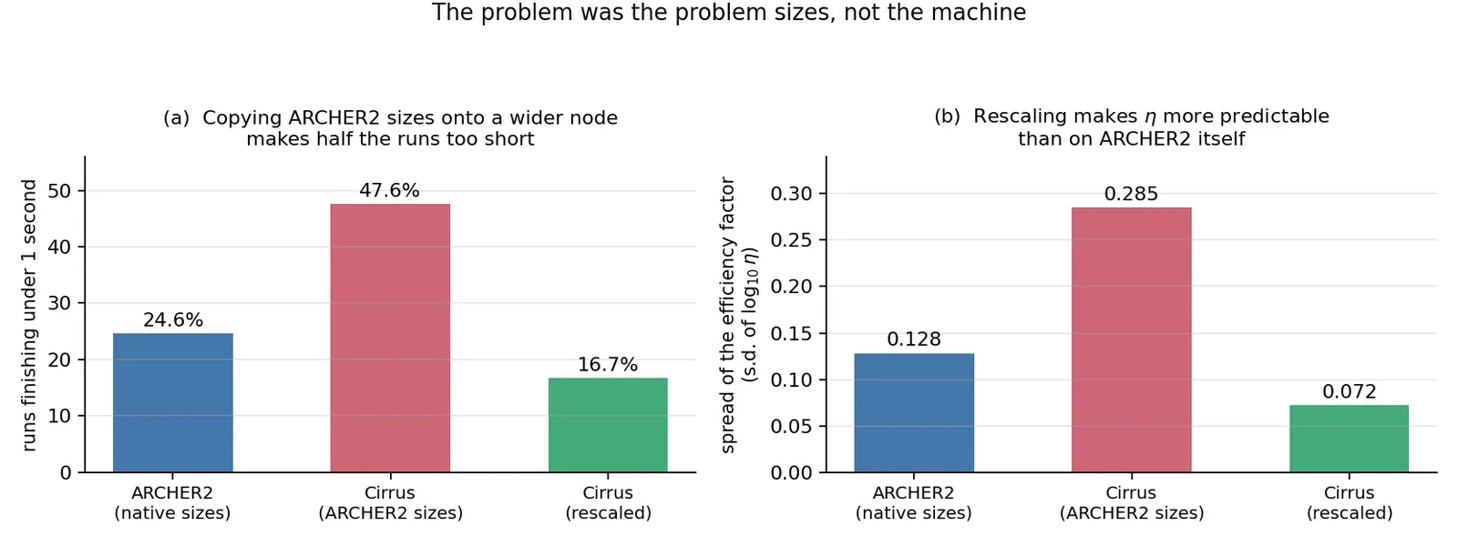
Left: copying ARCHER2’s sizes onto a wider node pushed nearly half the runs under a second. Right: what that did to the quantity the models have to predict. Rescaling brings the spread below ARCHER2’s own.

The distributional result is unambiguous and is the point of the experiment. The spread of $\eta$, its standard deviation, falls from 0.285 to 0.072 (below even ARCHER2’s 0.128), and sub-second runs fall from 47.6% to 16.7%. Nothing changed but the problem sizes.

Cirrus is not intrinsically harder to model. The fixed-size campaign was a badly designed experiment on it, because holding sizes constant while moving to a node twice as wide guarantees short runs.

The mechanism is visible directly:

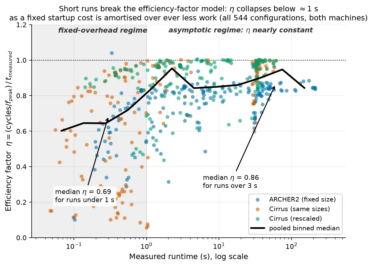
Above a second, the efficiency factor is nearly constant and a single scalar describes it well. Below a second it falls apart - fixed per-run cost the counted cycles never see, amortised over less and less work.

So $\eta$ is a property of how much work the run does, and not a property of the hardware. This generalises well beyond my campaign: any benchmark campaign whose runs fall below roughly one second will produce an unmodellable efficiency distribution regardless of the machine, and per-rank problem sizing of the kind HPCG uses avoids it.

The modelling consequence is weaker than the distributional one, and the two should not be allowed to carry each other. On the fixed-size Cirrus data the forest’s pooled median of 1.1863 sits above the constant’s 1.1663, but the paired test puts the forest ahead ($p = 0.0402$). On the rescaled data the forest at 1.0603 is nominally ahead of 1.0617 and that difference is not significant ($p = 0.366$).

The intervention moved the distribution decisively and left the model-versus-constant contrast ambiguous in both datasets. What is established is the causal claim about run length, not a claim that rescaling restores the models’ advantage. Rescaling made the task easier for every method, including the one with no parameters.

Pricing the circularity

Saying a method is circular is a criticism. Measuring what the circularity is worth is a result, and the second is far more useful.

So I set up the situation a procurement panel is actually in. An application has been profiled in full on the machine you own (ARCHER2), and a machine you do not own (Cirrus) is described only by datasheet facts: clock, memory bandwidth, core count and processor generation. Nothing measured on Cirrus appears anywhere in the predictor, meaning no Cirrus counters, no Cirrus runtimes and no Cirrus $\eta$. Validation is still leave-one-application-out, so the predictor faces an unseen application on an unmeasured machine simultaneously.

This differs from the previous section, where I transferred a model between machines but still measured the target (the Cirrus cycle count was available at test time). Here that measurement is removed entirely. The previous section asks “does a model trained elsewhere still work here?” This one asks “can you predict a machine you have never run on?”, which is the question the feasibility study actually posed and a strictly harder one.

The two italicised rows are reference points rather than competitors. The circular row is the same method with one change (the Cirrus cycle count handed back to it), so the gap between it and the best non-circular row measures exactly what the target-run counter is worth. It is a ceiling, since obtaining that counter means having run the job. The oracle row fits a single constant speedup on the test application’s own Cirrus data, which could never be done in practice, but it answers a useful question. If someone simply told you the right per-application speedup and nothing else, how well would you do?

The best non-circular predictor reaches 1.556 against a circular ceiling of 1.129.

Stated in terms of excess error (how far above a perfect 1.000 a prediction sits, since the metric cannot go below 1), removing the target-run counter grows the excess from 0.129 to 0.556, a factor of 4.3.

In terms a user would recognise, with one instrumented run of the job on the target machine, a typical prediction is out by about 13%, and without it, about 56%. That is the price of not having run the job, and putting a number on it was the point of the experiment.

How the learned predictors compare with plain arithmetic

This depends on how applications are weighted, and both readings belong in the record.

Pooled over the 166 configurations, the best learned predictor at 1.556 is nominally ahead of the 1.608 clock rescale but not significantly (it wins 94 of 166 at $p = 0.99$). That pool is dominated by HPCG, which supplies 44 rows and is the one application where clock rescaling wins outright (1.395 against 2.810).

Weighting the six applications equally inverts the picture, giving 1.653 against 1.990, with the learned predictor ahead on five of six and losing only on HPCG.

So RQ3’s negative is narrower than a flat statement of it. On a row-weighted pool the learned predictor does not significantly beat arithmetic, and that outcome is an artefact of one application’s weight. Per application it usually does, by a wide margin, and it fails badly on the single code whose cycle count behaves least like the others.

The uncomfortable row

A single constant speedup per application (one scalar, fitted on the test application itself and so not achievable, but requiring no counters at all) reaches a median of 1.130, matching the circular ceiling’s 1.129 and beating it in the tail (p90 1.669 against 3.601).

The entire counter pipeline, run on the target machine, buys nothing over one number per application.

That is uncomfortable, and it is the clearest statement of what the project found: the transferable signal in these counters is coarse and per-application, not fine-grained and microarchitectural.

The reason is visible in the cycle counts. If the cycle count were a machine-independent property of the work, its ratio between machines would be roughly constant and projection would reduce to a clock correction. It is not. The ratio has median 0.651, with per-application medians from 0.378 for LULESH to 1.666 for HPCG - a spread of 4.4× across applications for the same source code doing the same work. A model trained on ARCHER2 counters has no way to anticipate that.

One structural limitation bounds this whole experiment. With one target machine, the four static specification features are constant across every row by construction, hence the experiment cannot distinguish “ARCHER2 counters do not project onto Cirrus” from “static machine descriptions were never given a chance.” A third platform would separate the two.

---

Part IV. What it means

The overfitting warning, revisited

My supervisor warned early that the model would be prone to overfitting. He was right, but the mechanism was not the one either of us had in mind.

Overfitting is what happens when a model with enough flexibility learns the particular examples it was shown rather than the pattern behind them, scoring beautifully on training data and poorly on anything else, having memorised rather than generalised. I guarded against overfitting to rows from the start, by holding out whole applications.

The problems that actually materialised were quieter, and each was a variety of the same underlying fault: information about the test data reaching a decision it should not have influenced.

Overfitting to the folds. I chose hyperparameters by looking at leave-one-application-out results, trying architectures and adopting whichever scored best on the held-out applications. Those applications were supposed to be untouched, so the score is optimistic by however much the choice borrowed. Interestingly it made the model slightly worse rather than better, because a single fold-wide choice loses more than the leaked information gains.

Leakage through structure. I added binary indicator columns marking which counters were missing, expecting them to help the model distinguish absent from average. Each application turned out to have a unique missingness signature, so the columns functioned as a one-hot application label (a set of columns that between them name which application a row came from), which is precisely the fact leave-one-application-out is meant to withhold.

Aggregate accuracy barely moved. The held-out STREAM fold degraded from 1.096 to 1.552.

Pseudo-replication, which inflated the sample count while hollowing out the feature matrix.

Each of these was caught by looking at per-application results, and none would have been caught by an aggregate metric. The transferable lesson is that with leave-one-group-out validation, the per-group breakdown is where the failures live, and not a diagnostic extra.

Answering the four questions

RQ1 - can runtime be predicted from counters for unseen applications? No as posed, and yes in a restricted sense. The figures reconstruct a runtime whose cycle count has already been measured, rather than predicting an unrun execution. Within that scope the margin is measured (a random forest reaches 1.054 pooled, or 1.058 macro-averaged, against a zero-parameter constant at 1.065 and 1.111). The gain is large on five applications and a regression on three. At configuration granularity it is significant ($p = 1.4 \times 10^{-4}$). At the application granularity the validation protocol itself treats as independent, it is five wins to three and not significant ($p \approx 0.36$).

The defensible claim is that the effect is consistent in direction, materially large on most applications, and not established at the coarser unit.

RQ2 - where does the accuracy come from? This produced the central result. Across a five-rung ladder the cycle count contributes 100.8% of the total improvement and the remaining twenty features 0.2% pooled. Part of that dominance is definitional, and what the ladder measures beyond the definition is how little of the residual the counters recover. Free job metadata performs worse than a constant, only the complete five-run campaign beats that constant, and a single fitted speedup per application matches the whole pipeline.

RQ3 - does it transfer to a second machine? A qualified yes on transfer and a no on projection. Transferred models are worse in absolute terms than models that stay home, but going ARCHER2 → Cirrus they beat their own same-fold constant ($p = 0.006$), while in the reverse direction they do not. Whether what remains beats a clock-ratio rescale depends on weighting. The cycle count is not machine-invariant, with per-application ratios spanning a factor of four, and that is what defeats projection.

Cirrus’s apparent difficulty was experimental design rather than hardware: rescaling the problems for the wider node narrowed the spread of $\log_{10}\eta$ fourfold and cut sub-second runs by two thirds.

RQ4 - can it predict configurations that have not been run? No. The learned models are behind a two-parameter fit on the target’s own cheap runs at all three scale thresholds. They beat a constant, but the comparison that matters is the cheap alternative a practitioner would actually use. Restricting training to small scales costs essentially nothing, so the failure is not scale extrapolation, and the models were simply never ahead of a per-application straight line at any scale.

What a practitioner should actually do

The negative results have a constructive reading, and I would rather end on it than on the complaints.

For the runtime of an unrun configuration of a code you already have, run it two or three times at small core counts and fit a straight line. That beat every learned model here, needs no counters and no training set, and costs a few minutes of allocation.

For a code on a machine you do not own, having profiled it on one you do, fit a single scalar speedup per application. It matched the entire counter apparatus.

Counters earn their cost in the remaining case: explaining why a run took the time it did, once the run exists. There they are genuinely informative.

So my advice is to keep collecting counters, and to stop expecting them to substitute for a cheap run of the code in question.

What the modelling buys over reading the profiles directly

The apparatus consumes five profiles per configuration, so it is fair to ask what the modelling adds to simply reading them. It adds three things, and only three.

It generalises across configurations: a profile describes the run that produced it, whereas a fitted $\eta$ transfers to configurations that were never profiled, which is what leave-one-application-out tests. It compresses twenty-one counters into one interpretable scalar with a physical meaning. And it makes the accuracy falsifiable (the ladder exists precisely to say how much of that accuracy the counters earn rather than asserting it).

What it does not buy is a runtime for a job you have not run. For that, a profile and a model are equally useless, because both require the execution.

Which counters point at hardware improvements

A natural use for a fitted model is to read off which measured quantities matter most, and hence which hardware changes would pay.

That reading is available, but only after merging, for the reasons above. Once it is read correctly, the signal that survives is coarse. Stall fractions and arithmetic intensity carry most of what the counters contribute, and the twenty features beyond the cycle count together move the pooled median by 0.2%.

The honest answer to “which hardware improvement would help?” is that this apparatus is not sensitive enough to say. A study designed to answer it would need to vary the hardware rather than the code.

What the 4.3 factor means in practice

For the procurement scenario that motivates this work, the price is the difference between a prediction good enough to rank two machines and one good enough only to place them within a factor of two of each other.

A panel choosing between architectures on a 20% performance difference would not be served by it. A panel sizing an allocation to the nearest factor of two would. Stating the number is more useful than either promising projection or dismissing it.

What I got wrong

Several claims I made earlier in the project did not survive scrutiny. The corrected numbers are the ones quoted throughout this article, and the superseded results stayed in my working repository rather than being deleted, each with a note explaining what was wrong with it. The harness, the parsed measurements and the code behind the final numbers are at the bottom of this page. It’s there to check the working against, or to take the harness from for a study of your own.

I found five defects in my own analysis, and the most instructive one generalises beyond this study, so it gets the space.

The retraction

At one point I reported that a particular energy-derived feature was overwhelmingly the strongest predictor in the model, with a random-forest importance of 0.509, more than every other feature combined. I was ready to offer it as the project’s clearest novelty claim.

It was an artefact of the counter rotation.

Only five counters fit at once, so features arrive from five different runs and the assembled matrix has a structured missingness pattern. RAPL energy sits on separate registers, so it was present in every counter set while everything else was present in one. Impurity-based feature importance does not distinguish “this feature explains a lot” from “this feature was observed a lot”. Imputation makes the missing columns uninformative by construction, so importance mass migrates to whichever counter happened to be always available.

On the corrected, merged data that feature ranks 15th of 21, with an importance of 0.008. The corrected leaders are the analytic time (0.376), FLOPs per instruction (0.134), instructions per rank (0.112) and the FP stall fraction (0.077).

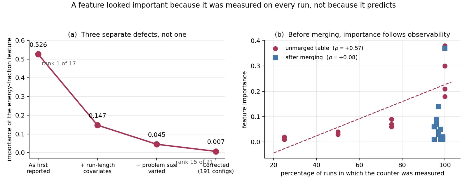
Left: three compounding defects, each stripping away part of the claim. Right: the mechanism - before merging, importance tracks how often a counter was observed rather than how much it explains.

Three separate defects compounded: no run-length covariate on the original 40-row table, one problem size per application confounding identity with signature, and the structural missingness of the 815-row unmerged table.

The general warning is that impurity feature importance is not interpretable on a feature matrix assembled by counter multiplexing. Any rotated-counter campaign that reports feature importances without merging first is reporting its own sampling schedule. Given how common counter rotation is (it is forced on you by hardware on essentially every modern processor), I suspect this is not a rare mistake.

The other four

The baseline was a strawman. An earlier version reported a 20% gain over a baseline that predicted the mean of a left-skewed target, one whose values pile up at the high end with a tail to the low, while the error metric is minimised by the median. Every number here uses the corrected median-constant baseline.

The two platforms were never matched. 166 configurations, not 191, exist on both machines. On the paired subset both tree models beat the constant within Cirrus, which reverses the published claim that Zen 5 is genuinely harder to predict.

Seven of twenty-eight direction labels were backwards. Every script ran a paired Wilcoxon test and then labelled the direction by comparing two independent medians, but median(a) − median(b) is not median(a − b). Because the error distributions are right-skewed, a model can shift most pairs down while a few large-error pairs hold its own marginal median up. Every one of the seven flips ran the same way, from “worse” to “model better”, hence the old labelling was systematically pessimistic about the models.

Four decimal places were never justified. The same nominal experiment was published as 1.054, 1.055, 1.0548 and 1.0554. All four were reproduced exactly and are fully explained by two incidental implementation differences (feature column order, and a saturation effect in one script’s scaler), and neither is a difference in method or data. Meanwhile the seed spread over ten random states is 0.0158, five times the entire implementation spread. Quote two decimals with an interval.

Limitations

The circularity is fundamental rather than incidental: the dominant predictor is measured on the target run, and no quantity of additional data changes that. Only a different predictor would.

Beyond that:

CrayPat reports rank 0 only, so rank imbalance is invisible to the features and lives in the residual. The severity is not constant. At one rank, rank 0 is the whole job, and at 128 ranks it is 0.8% of it, so the bias varies systematically along the core-count axis, which is one of the axes being modelled. A control run with counters on several ranks would have bounded it.

Every runtime here is instrumented and no uninstrumented baseline was collected, so CrayPat’s overhead sits inside the target variable.

Both platforms are AMD Cray EX systems, so nothing here supports transfer to a materially different architecture. The Zen 2 stall and L3 events have no Zen 5c equivalent, which is why cross-platform work uses 14 features rather than 21.

GROMACS and OpenFOAM remain at one problem size each and were not run on Cirrus, so they are excluded from every cross-platform result.

Everything is single-node by design.

Three defects in the sweep harness deserve naming individually, because they bear on how the per-application results should be read.

STREAM did not run threaded in the expanded campaign. The original harness launched it correctly for an OpenMP-only code. The expanded harness set one thread globally and launched every code with one task per core. Since STREAM contains no MPI, this ran $N$ independent single-threaded copies rather than one $N$-threaded job. The signature is unmistakable (rank-0 instruction count constant to four significant figures across all eight core counts), hence STREAM’s expanded configurations carry no scaling signal.

HPCG runs 1.5 times the iterations on Cirrus. The ARCHER2 harness writes 20 CG iterations and the Cirrus harness 30, while the cross-platform join matches on problem size and core count without matching iteration count. Cirrus therefore performs half as much work again on the 44 of 166 matched configurations HPCG contributes, which accounts for the direction and much of the magnitude of its outlying cycle ratio of 1.666 against 0.378–0.827 for every other application. The pooled cross-platform comparison should be read as contaminated by this, and the macro-average as the reliable summary. The qualitative conclusion survives, because the five uncontaminated applications still span a factor of 2.2.

The two ARCHER2 sweeps overlap on sixteen configurations (eight of HPCG and eight of STREAM), and the merge key does not include which campaign a run came from. Those sixteen medians therefore pool runs from two harnesses with different iteration counts and different parallelism models. Sixteen of 191 configurations are affected, but HPCG supplies 45 rows and dominates the pooled medians. Recomputing with campaign in the merge key would settle how much it moves. That was not done, and it is the first thing I would check in any continuation.

What I’d do differently

Spend the profiling budget on more applications and fewer configurations each. The learning curve is unambiguous, and I found it too late to act on. Profiling each code at eight core counts and four sizes bought density the model had stopped using.

Size the Cirrus problems for the Cirrus node. I kept problem sizes identical to ARCHER2’s so both machines ran the same work, which is the natural way to make a fair comparison. But on a node more than twice as wide, that pushed nearly half the runs below a second, where fixed overhead dominates and the efficiency factor collapses. Comparability and predictability pulled against each other, and I picked the wrong one without noticing there was a choice.

Collect an uninstrumented repeat set. Five runs per configuration gave five wall-clock samples, but each carried different instrumentation, so their spread mixes run-to-run variance with instrumentation overhead and cannot be read as either. That spread is the dominant uncertainty in the whole campaign, and separating it would have cost one extra run per configuration.

Build the measurement ladder first, not last. This is the big one. Constructing it cost about a day, and it reframed the entire project, turning “here is an accuracy number” into “here is which measurement earned the accuracy, and here is what the indispensable one costs.” Every interesting result in this article is downstream of that reframing, and I built the thing in the final months.

Where I would take it next

The clock-ratio rescale that no learned model significantly beat is the obvious starting point, since it is nearly free, and modelling the cycle-count ratio between machines directly is the natural extension. So is recovering an instruction mix without execution, by static analysis of the binary, which would attack the circularity at its root rather than pricing it.

Beyond that, a third platform of a genuinely different architecture (Intel, Arm, or something with high-bandwidth memory) would test whether $\eta$ carries any architecture-independent meaning, which two AMD Cray EX systems cannot. Collecting counters from ranks other than rank 0 would make load imbalance visible to the features rather than leaving it in the residual. RAPL energy, collected throughout at no additional cost but used only as a feature, is a second prediction target the existing dataset already supports.

---

The finding I would most want someone to take away is that the variation that mattered was in what got measured, not in what got fitted to it, and it is not specific to counters.

Three estimator families landed within 0.02 of each other (two of them approximating functions in structurally unrelated ways), while the gap between having one particular counter and not having it was a factor of 4.3. I spent a good deal of this project tuning models, and almost none of that effort moved the result.

The ladder is what moved it, and a ladder is just the discipline of changing one thing at a time and scoring everything the same way.

---

Appendix. What was actually measured

Every counter collected

There are twenty counters on ARCHER2, of which eleven are also available on Cirrus. That intersection is what carries every cross-platform result above: the Zen 2 uncore L3 and RAPL energy events have no Cirrus equivalent exposed through CrayPat, and the branch, vector and FMA events were unavailable on ARCHER2’s Rome cores.

Stall counters are abbreviated from their DISPATCH_RESOURCE_STALL_CYCLES_1 prefix, and the two L2 traffic events from REQUESTS_TO_L2_GROUP1.

The rotation schedule

Five counters fit at once, so a wide feature set needs repeated execution. This is the schedule that produced the twenty:

The RAPL and Zen L3 events at the foot use separate registers, so they are collected on every run without consuming any of the five slots. TOT_CYC appears in four sets because it normalises whatever else that run measures, so the sets are not disjoint, and the union is twenty counters rather than twenty-three.

BR_INS and BR_MSP were requested in set E but returned no values on the Rome cores, which is why they appear in the schedule above but not as ARCHER2 counters in the table before it.

The derived features

The raw counters never enter a model directly. What enters is always a ratio, so that magnitude divides out and only the character of the execution remains. These are the ones whose definitions are not obvious from the name:

Here $C$ is cycles and $I$ instructions, and the 64 in the arithmetic-intensity row converts L3 misses to bytes at one cache line each.

That core energy fraction row is the feature I once reported at 0.509 importance and had to retract. It is included here rather than quietly dropped, because the definition is fine - it was the inference drawn from it that was wrong.